TensorFlow - 04.Logistic Regression

Logistic Regression

view jupyter notebook code

List of Tensorflow 2.0 Tutorials

• TF2.0 - 01.Simple Linear Regression
• TF2.0 - 02.Linear Regression and How to minimize cost
• TF2.0 - 03.Multiple Linear Regression
• TF2.0 - 04.Logistic Regression
• TF2.0 - 05.Multinomial Classification
• TF2.0 - 06.Iris Data Classification

Now let’s create a classification model for two categories.

(Review) Multiple Linear Regression

Hypothesis

\[H(X) = XW\]

Cost Function

\[Cost(W) = {1 \over m} {\sum_{i=1}^m} (H(X_i)-Y_i)^2\]

Minimizing Cost

\[W_{new} = W_{old} - \alpha {\partial \over {\partial W}} Cost(W)\]

Logistic Regression

Hypothesis

\[{H(X)} = {1 \over {1+ e^{-XW}}}\]

Cost Function

\[Cost(W) = {1 \over m} {\sum_{i=1}^m c(H(x_{i}), y_{i})}\]

Cross Entropy in Logistic Classification

\[c(H(x), y) = \begin{cases}-log(H(x)) : y=1 \\ -log(1-H(x)) : y=0\end{cases} = -y log(H(x)) - (1-y) log(1-H(x))\]

Minimizing Cost

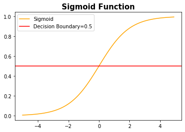
\[W_{new} = W_{old} - \alpha {\partial \over {\partial W}} Cost(W)\]

Sigmoid Function, Hypothesis of Logistic Regression Model

In the logistic regression model, Hypothesis in the Linear Regression Model is applied to the Sigmoid function.

\[Sigmoid(x) = {1 \over {1+e^{-x}}}\]

import numpy as np
import matplotlib.pyplot as plt

x = np.arange(-5, 5, 0.1)
y = 1/(1+np.exp(-x))

plt.title('Sigmoid Function', size=15, weight='bold')
plt.plot(x,y,color='orange', label='Sigmoid')
plt.axhline(0.5, color='red', label='Decision Boundary=0.5')
plt.legend(loc='upper left')
plt.show()

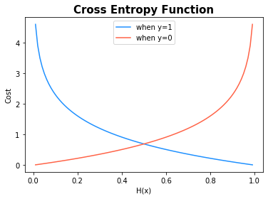
Cross Entropy Function, Cost of Logistic Regression Model

You can see that it uses different cost functions depending on the class of the actual y value.

\[c(H(x), y) = \begin{cases}-log(H(x)) : y=1 \\ -log(1-H(x)) : y=0\end{cases} = -y log(H(x)) - (1-y) log(1-H(x))\]

x = np.arange(0.01, 1, 0.01)
y1 = -np.log(x)
y0 = -np.log(1-x)

plt.title('Cross Entropy Function', size=15, weight='bold')
plt.plot(x, y1, color='dodgerblue', label='when y=1')
plt.plot(x, y0, color='tomato', label='when y=0')
plt.xlabel('H(x)')
plt.ylabel('Cost')
plt.legend(loc='upper center')
plt.show()

Implement

import tensorflow as tf
import numpy as np
import pandas as pd
import seaborn as sns
import matplotlib.pyplot as plt

print("TensorFlow Version: %s" % (tf.__version__))

TensorFlow Version: 2.0.0

Data

# Data for train
x_train = np.array([[1., 1.],
                   [1., 2.],
                   [2., 1.],
                   [3., 2.],
                   [3., 3.],
                   [2., 3.]],
                   dtype=np.float32)

y_train = np.array([[0.],
                   [0.],
                   [0.],
                   [1.],
                   [1.],
                   [1.]],
                   dtype=np.float32)

# Data for test
x_test = np.array([[3., 0.],
                   [4., 1.]],
                   dtype=np.float32)

y_test = np.array([[0.],
                   [1.]],
                   dtype=np.float32)

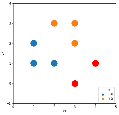
Visualization

There are two classes, blue and orange. We will classify the new data, red data, into one of two classes, blue and orange.

df = pd.DataFrame(x_train, columns=['x1','x2'])
df['y'] = y_train

df_test = pd.DataFrame(x_test, columns=['x1','x2'])
df_test['y'] = y_test

plt.figure(figsize=(6,6))
sns.scatterplot(x='x1', y='x2', hue='y', data=df, s=500)
sns.scatterplot(x='x1', y='x2', color='red', data=df_test, s=500)
plt.xlim(0, 5)
plt.ylim(-1, 4)
plt.legend(loc='lower right')
plt.show()

Initializing Weights

# Weights
tf.random.set_seed(2020)
W = tf.Variable(tf.random.normal([2, 1], mean=0.0))
b = tf.Variable(tf.random.normal([1], mean=0.0))

print('# Weights: \n', W.numpy(), '\n\n# Bias: \n', b.numpy())

# Weights:
 [[-0.10099822]
 [ 0.6847899 ]]

# Bias:
 [0.38414612]

Train the model

# Learning Rate
learning_rate = 0.01

# Hypothesis and Prediction Function
def predict(X):
    z = tf.matmul(X, W) + b
    hypothesis = 1 / (1 + tf.exp(-z))
    return hypothesis

# Training
for i in range(2000+1):

    with tf.GradientTape() as tape:

        hypothesis = predict(x_train)
        cost = tf.reduce_mean(-tf.reduce_sum(y_train*tf.math.log(hypothesis) + (1-y_train)*tf.math.log(1-hypothesis)))        
        W_grad, b_grad = tape.gradient(cost, [W, b])

        W.assign_sub(learning_rate * W_grad)
        b.assign_sub(learning_rate * b_grad)

    if i % 400 == 0:
        print(">>> #%s \n Weights: \n%s \n Bias: \n%s \n cost: %s\n" % (i, W.numpy(), b.numpy(), cost.numpy()))

>>> #0
 Weights:
[[-0.11992227]
 [ 0.66358066]]
 Bias:
[0.36538637]
 cost: 4.759439

>>> #400
 Weights:
[[0.61899596]
 [0.7487086 ]]
 Bias:
[-2.3262427]
 cost: 2.1940103

>>> #800
 Weights:
[[1.058025 ]
 [1.0836021]]
 Bias:
[-3.9347079]
 cost: 1.4598237

>>> #1200
 Weights:
[[1.3448476]
 [1.3511039]]
 Bias:
[-5.073361]
 cost: 1.094249

>>> #1600
 Weights:
[[1.562529 ]
 [1.5643576]]
 Bias:
[-5.95332]
 cost: 0.8763469

>>> #2000
 Weights:
[[1.7395078]
 [1.7401232]]
 Bias:
[-6.670953]
 cost: 0.7315402

Predict

The red data is well categorized.

hypo = predict(x_test)
print("Prob: \n", hypo.numpy())
print("Result: \n", tf.cast(hypo > 0.5, dtype=tf.float32).numpy())

Prob:
 [[0.18962799]
 [0.8836236 ]]
Result:
 [[0.]
 [1.]]

Accuracy

Both observations are well categorized and the classification accuracy is 100%.

def acc(hypo, label):
    predicted = tf.cast(hypo > 0.5, dtype=tf.float32)
    accuracy = tf.reduce_mean(tf.cast(tf.equal(predicted, label), dtype=tf.float32))
    return accuracy

accuracy = acc(predict(x_test), y_test).numpy()
print("Accuracy: %s" % accuracy)

Accuracy: 1.0

List of Tensorflow 2.0 Tutorials

• TF2.0 - 01.Simple Linear Regression
• TF2.0 - 02.Linear Regression and How to minimize cost
• TF2.0 - 03.Multiple Linear Regression
• TF2.0 - 04.Logistic Regression
• TF2.0 - 05.Multinomial Classification
• TF2.0 - 06.Iris Data Classification