제2장 : 통계 분석
먼저 데이터 분석을 수행할 환경의 경로를 설정합니다.
# Working Directory
setwd('C:/Users/wooil/Documents/GitHub/ADP')
getwd()
‘C:/Users/wooil/Documents/GitHub/ADP’
제2절 기초 통계 분석
1. 기술 통계
print(head(iris))
summary(iris)
  Sepal.Length Sepal.Width Petal.Length Petal.Width Species
1          5.1         3.5          1.4         0.2  setosa
2          4.9         3.0          1.4         0.2  setosa
3          4.7         3.2          1.3         0.2  setosa
4          4.6         3.1          1.5         0.2  setosa
5          5.0         3.6          1.4         0.2  setosa
6          5.4         3.9          1.7         0.4  setosa


  Sepal.Length    Sepal.Width     Petal.Length    Petal.Width
 Min.   :4.300   Min.   :2.000   Min.   :1.000   Min.   :0.100
 1st Qu.:5.100   1st Qu.:2.800   1st Qu.:1.600   1st Qu.:0.300
 Median :5.800   Median :3.000   Median :4.350   Median :1.300
 Mean   :5.843   Mean   :3.057   Mean   :3.758   Mean   :1.199
 3rd Qu.:6.400   3rd Qu.:3.300   3rd Qu.:5.100   3rd Qu.:1.800
 Max.   :7.900   Max.   :4.400   Max.   :6.900   Max.   :2.500
       Species
 setosa    :50
 versicolor:50
 virginica :50
# 평균, 중앙값, 표준편차, 분산, 1사분위수, 2사분위수, 3사분위수, 최댓값, 최솟값
print(mean(iris$Sepal.Length))
print(median(iris$Sepal.Length))
print(sd(iris$Sepal.Length))
print(var(iris$Sepal.Length))
print(quantile(iris$Sepal.Length, 1/4))
print(quantile(iris$Sepal.Length, 2/4))
print(quantile(iris$Sepal.Length, 3/4))
print(max(iris$Sepal.Length))
print(min(iris$Sepal.Length))
[1] 5.843333
[1] 5.8
[1] 0.8280661
[1] 0.6856935
25%
5.1
50%
5.8
75%
6.4
[1] 7.9
[1] 4.3
# MASS 패키지에 내장된 28가지 종의 동물 뇌의 무게와 몸무게 데이터
install.packages("MASS")
library(MASS)
Installing package into 'C:/Users/wooil/Documents/R/win-library/3.6'
(as 'lib' is unspecified)


package 'MASS' successfully unpacked and MD5 sums checked

The downloaded binary packages are in
	C:\Users\wooil\AppData\Local\Temp\RtmpeQ9CHr\downloaded_packages
data("Animals")
print(head(Animals))
                    body brain
Mountain beaver     1.35   8.1
Cow               465.00 423.0
Grey wolf          36.33 119.5
Goat               27.66 115.0
Guinea pig          1.04   5.5
Dipliodocus     11700.00  50.0
summary(Animals)
      body              brain
 Min.   :    0.02   Min.   :   0.40
 1st Qu.:    3.10   1st Qu.:  22.23
 Median :   53.83   Median : 137.00
 Mean   : 4278.44   Mean   : 574.52
 3rd Qu.:  479.00   3rd Qu.: 420.00
 Max.   :87000.00   Max.   :5712.00
# 바디와 브레인의 사분위수 출력
print(quantile(Animals$body))
print(quantile(Animals$brain))
       0%       25%       50%       75%      100%
    0.023     3.100    53.830   479.000 87000.000
      0%      25%      50%      75%     100%
   0.400   22.225  137.000  420.000 5712.000
# 브레인/바디로 계산한 Ratio 변수 생성
Animals$ratio = Animals$brain/Animals$body
print(head(Animals))
                    body brain       ratio
Mountain beaver     1.35   8.1 6.000000000
Cow               465.00 423.0 0.909677419
Grey wolf          36.33 119.5 3.289292596
Goat               27.66 115.0 4.157628344
Guinea pig          1.04   5.5 5.288461538
Dipliodocus     11700.00  50.0 0.004273504
회귀분석
1. 모형이 통계적으로 유의미한가?
F통계량을 확인한다. 유의수준 5% 하에서 F통계량의 p-값이 0.05보다 작으면 추정된 회귀식은 통계적으로 유의하다고 볼 수 있다.

2. 회귀계수들이 유의미한가?
해당 계수의 t통계량과 p-값 또는 이들의 신뢰구간을 확인한다.

3. 모형이 얼마나 설명력을 갖는가?
결정계수를 확인한다. 결정계수는 0에서 1값을 가지며, 높은 값을 가질수록 추정된 회귀식의 설명력이 높다.

4. 모형이 데이터를 잘 적합하고 있는가?
잔차를 그래프로 그리고 회귀진단을 한다.

5. 데이터가 아래의 모형 가정을 만족시키는가?

<가정>

- 선형성(독립변수의 변화에 따라 종속변수도 일정크기로 변화)
- 독립성(잔차와 독립변수의 값이 관련돼 있지 않음)
- 등분산성(독립변수의 모든 값에 대해 오차들의 분산이 일정)
- 비상관성(관측치들의 잔차들끼리 상관이 없어야 함)
- 정상성(잔차항이 정규분포를 이뤄야 함)
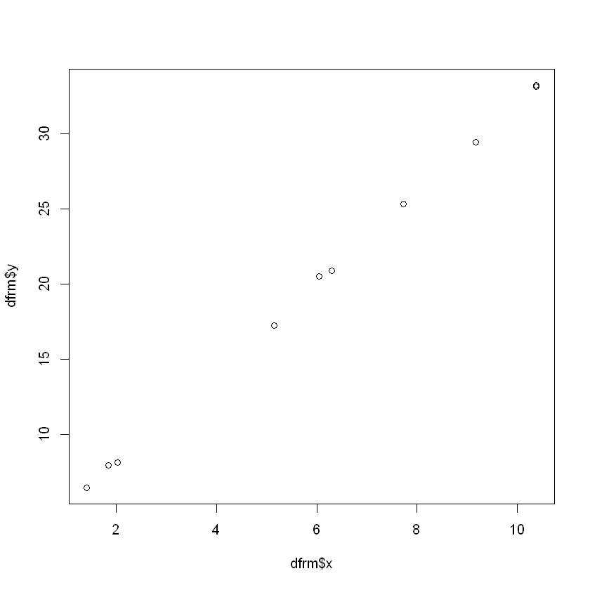
단순회귀분석
set.seed(2)
x = runif(10,0,11)
y = 2 + 3*x + rnorm(10, 0, 0.2)
dfrm = data.frame(x,y)
print(dfrm)
           x         y
1   2.033705  8.127599
2   7.726114 25.319934
3   6.306590 20.871829
4   1.848571  7.942608
5  10.382233 33.118941
6  10.378225 33.218204
7   1.420749  6.458597
8   9.167937 29.425272
9   5.148204 17.236677
10  6.049821 20.505909
plot(dfrm$x, dfrm$y)
m <- lm(y~x, data=dfrm)
m
Call:
lm(formula = y ~ x, data = dfrm)

Coefficients:
(Intercept)            x
      2.213        2.979
summary(m)
Call:
lm(formula = y ~ x, data = dfrm)

Residuals:
      Min        1Q    Median        3Q       Max
-0.311062 -0.118624 -0.002713  0.093296  0.272610

Coefficients:
            Estimate Std. Error t value Pr(>|t|)
(Intercept)   2.2133     0.1257   17.61 1.11e-07 ***
x             2.9786     0.0183  162.76 2.27e-15 ***
---
Signif. codes:  0 '***' 0.001 '**' 0.01 '*' 0.05 '.' 0.1 ' ' 1

Residual standard error: 0.1885 on 8 degrees of freedom
Multiple R-squared:  0.9997,	Adjusted R-squared:  0.9997
F-statistic: 2.649e+04 on 1 and 8 DF,  p-value: 2.272e-15
다중회귀분석
set.seed(2)

u=runif(10,0,11)
v=runif(10,11,20)
w=runif(10,1,30)

y=3 + 0.1*u + 2*v - 3*w + rnorm(10,0, 0.1)

dfrm = data.frame(y,u,v,w)
print(dfrm)
             y         u        v         w
1  -25.6647952  2.033705 15.97407 20.195064
2   -6.5562326  7.726114 13.15005 12.238937
3  -36.4858791  6.306590 17.84462 25.269786
4   12.4472764  1.848571 12.62738  5.364542
5    0.1638434 10.382233 14.64754 11.070895
6   -3.9124946 10.378225 18.68194 15.174424
7   26.6127780  1.420749 19.78759  5.328159
8   -3.9238295  9.167937 13.03243 11.354815
9  -53.0331805  5.148204 15.00328 28.916677
10  12.4387413  6.049821 11.67481  4.838788
m<-lm(y~u+v+w)
m
Call:
lm(formula = y ~ u + v + w)

Coefficients:
(Intercept)            u            v            w
     3.0417       0.1232       1.9890      -2.9978
summary(m)
Call:
lm(formula = y ~ u + v + w)

Residuals:
      Min        1Q    Median        3Q       Max
-0.188562 -0.058632 -0.002013  0.080024  0.143757

Coefficients:
             Estimate Std. Error  t value Pr(>|t|)
(Intercept)  3.041653   0.264808   11.486 2.62e-05 ***
u            0.123173   0.012841    9.592 7.34e-05 ***
v            1.989017   0.016586  119.923 2.27e-11 ***
w           -2.997816   0.005421 -552.981 2.36e-15 ***
---
Signif. codes:  0 '***' 0.001 '**' 0.01 '*' 0.05 '.' 0.1 ' ' 1

Residual standard error: 0.1303 on 6 degrees of freedom
Multiple R-squared:      1,	Adjusted R-squared:      1
F-statistic: 1.038e+05 on 3 and 6 DF,  p-value: 1.564e-14
결과
- F통계량:1.038e+05 p-값:1.564e-14 –> 유의수준 5% 하에서 추정된 회귀 모형이 통계적으로 매우 유의함.
- 결정계수 및 수정된 결정계수 모두 1로 이 회귀식이 데이터를 매우 잘 설명하고 있음.
- 회귀계수 u, v, w들의 p-값들도 0.01보다 작으므로 회귀계수의 추정치들이 유의수준 5% 하에서 통계적으로 유의함.
식이요법 방법을 적용한 닭에 대한 데이터
library(MASS)
data(ChickWeight)
print(head(ChickWeight))
  weight Time Chick Diet
1     42    0     1    1
2     51    2     1    1
3     59    4     1    1
4     64    6     1    1
5     76    8     1    1
6     93   10     1    1
1번 닭에게 식이요법 방법 1을 적용한 데이터만 조회해 Chick 변수에 할당
Chick = ChickWeight[ChickWeight$Diet==1 & ChickWeight$Chick==1,]
print(Chick)
   weight Time Chick Diet
1      42    0     1    1
2      51    2     1    1
3      59    4     1    1
4      64    6     1    1
5      76    8     1    1
6      93   10     1    1
7     106   12     1    1
8     125   14     1    1
9     149   16     1    1
10    171   18     1    1
11    199   20     1    1
12    205   21     1    1
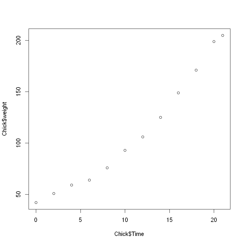
시간의 경과에 따른 닭들의 몸무게를 단순회귀분석 시행
model = lm(weight ~ Time, Chick)
summary(model)
Call:
lm(formula = weight ~ Time, data = Chick)

Residuals:
     Min       1Q   Median       3Q      Max
-14.3202 -11.3081  -0.3444  11.1162  17.5346

Coefficients:
            Estimate Std. Error t value Pr(>|t|)
(Intercept)  24.4654     6.7279   3.636  0.00456 **
Time          7.9879     0.5236  15.255 2.97e-08 ***
---
Signif. codes:  0 '***' 0.001 '**' 0.01 '*' 0.05 '.' 0.1 ' ' 1

Residual standard error: 12.29 on 10 degrees of freedom
Multiple R-squared:  0.9588,	Adjusted R-squared:  0.9547
F-statistic: 232.7 on 1 and 10 DF,  p-value: 2.974e-08
plot(Chick$Time, Chick$weight)
결과
추정된 회귀식
weight = 24.4654 + 7.9879*time
- F통계량:232.7 p-값:2.974e-08 –> 유의수준 5% 하에서 추정된 회귀 모형이 통계적으로 매우 유의함.
- 결정계수 또한 0.9588로 매우 노은 값을 보이므로 이 회귀식이 데이터를 96% 정도로 설명하고 있음.
- 회귀계수들의 p-값들도 0.05보다 매우 작으므로 회귀계수의 추정치들이 유의수준 5% 하에서 통계적으로 유의함.
해석
time이 1 증가할 때, weight이 7.99 만큼 증가한다.
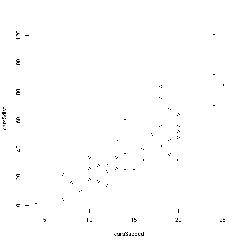
다항회귀분석
dist = a + bspeed + cspeed^2 + e
data(cars)
print(head(cars))
  speed dist
1     4    2
2     4   10
3     7    4
4     7   22
5     8   16
6     9   10
plot(cars$speed, cars$dist)
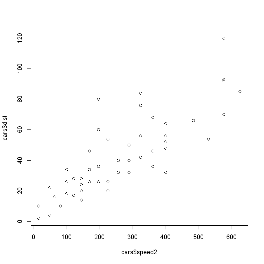
cars$speed2 = cars$speed^2
plot(cars$speed2, cars$dist)
model = lm(cars$dist~speed+speed2, cars)
model
Call:
lm(formula = cars$dist ~ speed + speed2, data = cars)

Coefficients:
(Intercept)        speed       speed2
    2.47014      0.91329      0.09996
summary(model)
Call:
lm(formula = cars$dist ~ speed + speed2, data = cars)

Residuals:
    Min      1Q  Median      3Q     Max
-28.720  -9.184  -3.188   4.628  45.152

Coefficients:
            Estimate Std. Error t value Pr(>|t|)
(Intercept)  2.47014   14.81716   0.167    0.868
speed        0.91329    2.03422   0.449    0.656
speed2       0.09996    0.06597   1.515    0.136

Residual standard error: 15.18 on 47 degrees of freedom
Multiple R-squared:  0.6673,	Adjusted R-squared:  0.6532
F-statistic: 47.14 on 2 and 47 DF,  p-value: 5.852e-12
결과
추정된 회귀식
dist = 2.47014 + 0.91329speed + 0.09996speed^2
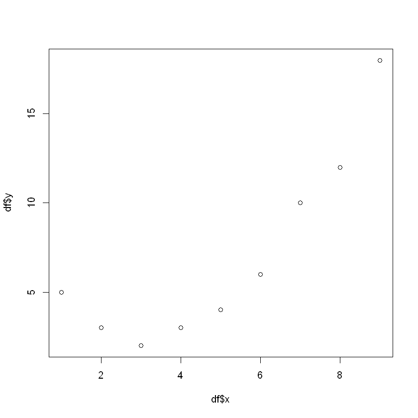
(예제) 적절한 회귀모형 탐색
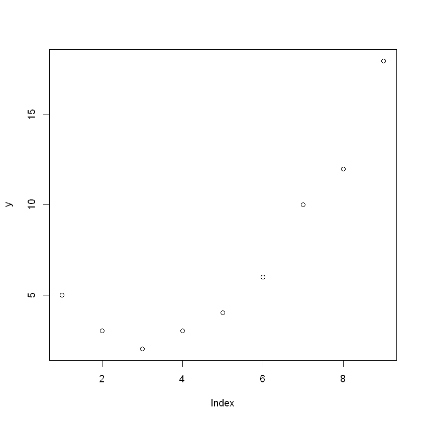
## Data 생성
x=c(1:9)
y=c(5,3,2,3,4,6,10,12,18)
df=data.frame(x,y)
print(df)
  x  y
1 1  5
2 2  3
3 3  2
4 4  3
5 5  4
6 6  6
7 7 10
8 8 12
9 9 18
## EDA
plot(df$x, df$y)  # 2차 함수 관계 파악
df$x2 = df$x^2    # x 제곱항 추가
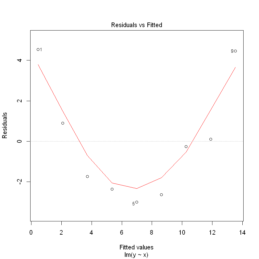
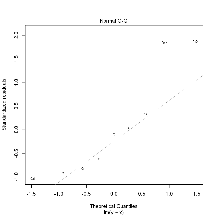
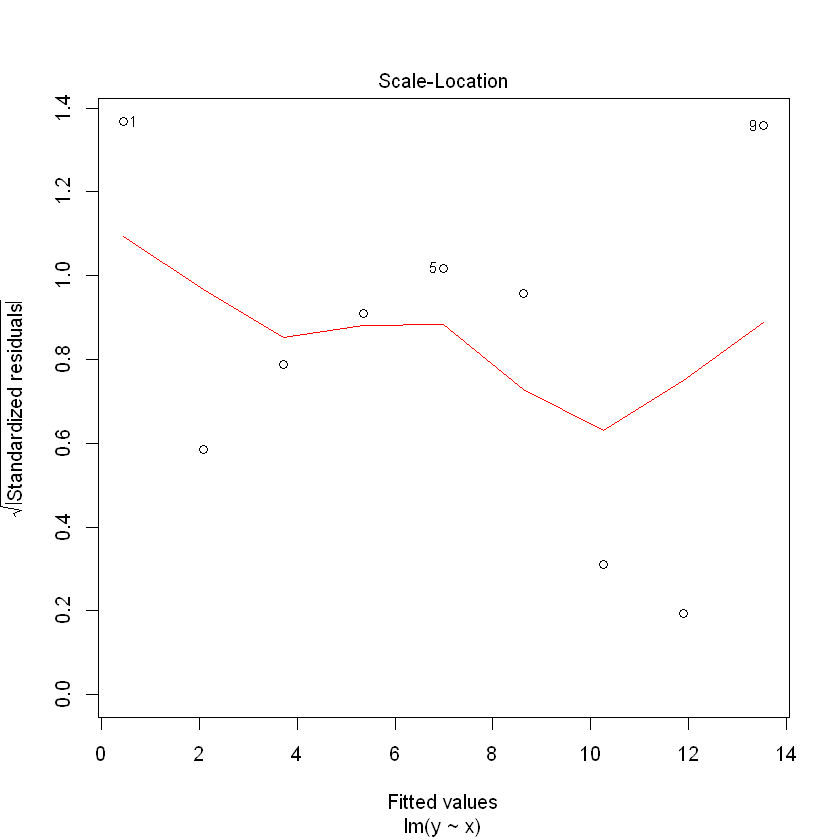
## 1) 제곱항 미포함 회귀식 적합
model1 = lm(y~x, df)
summary(model1)
plot(model1)
Call:
lm(formula = y ~ x, data = df)

Residuals:
    Min      1Q  Median      3Q     Max
-3.0000 -2.3667 -0.2667  0.9000  4.5333

Coefficients:
            Estimate Std. Error t value Pr(>|t|)
(Intercept)  -1.1667     2.2296  -0.523  0.61694
x             1.6333     0.3962   4.122  0.00445 **
---
Signif. codes:  0 '***' 0.001 '**' 0.01 '*' 0.05 '.' 0.1 ' ' 1

Residual standard error: 3.069 on 7 degrees of freedom
Multiple R-squared:  0.7083,	Adjusted R-squared:  0.6666
F-statistic: 16.99 on 1 and 7 DF,  p-value: 0.004446
(추정된 회귀식)
y = -1.1667 + 1.6333*x
설명력 : 70.83%
(회귀식 잔차도 해석)
잔차가 곡선 패턴을 가지므로 오차팡은 평균이 0이고 분산이 일정하다는 가정을 만족하지 않음.
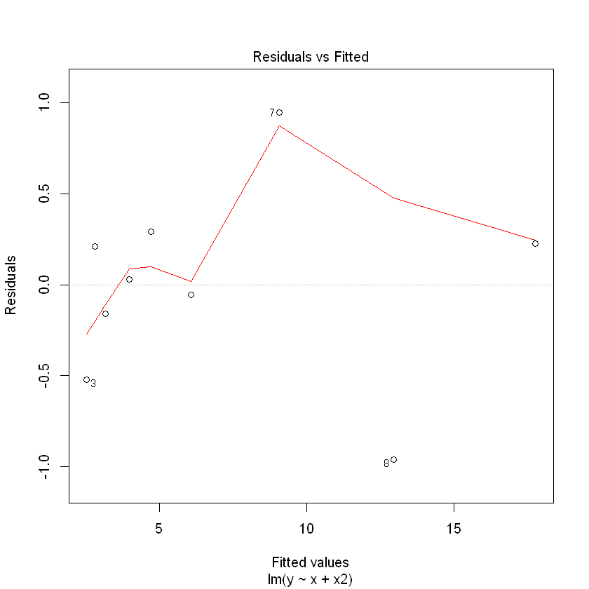
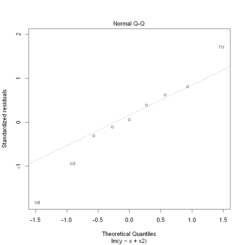
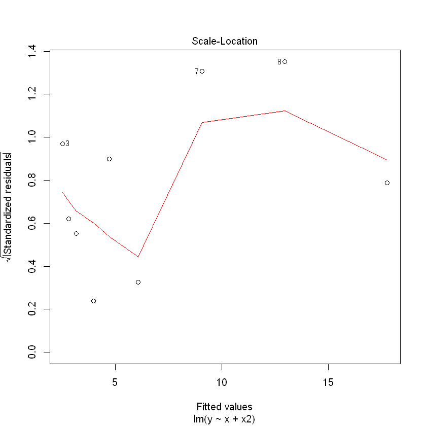
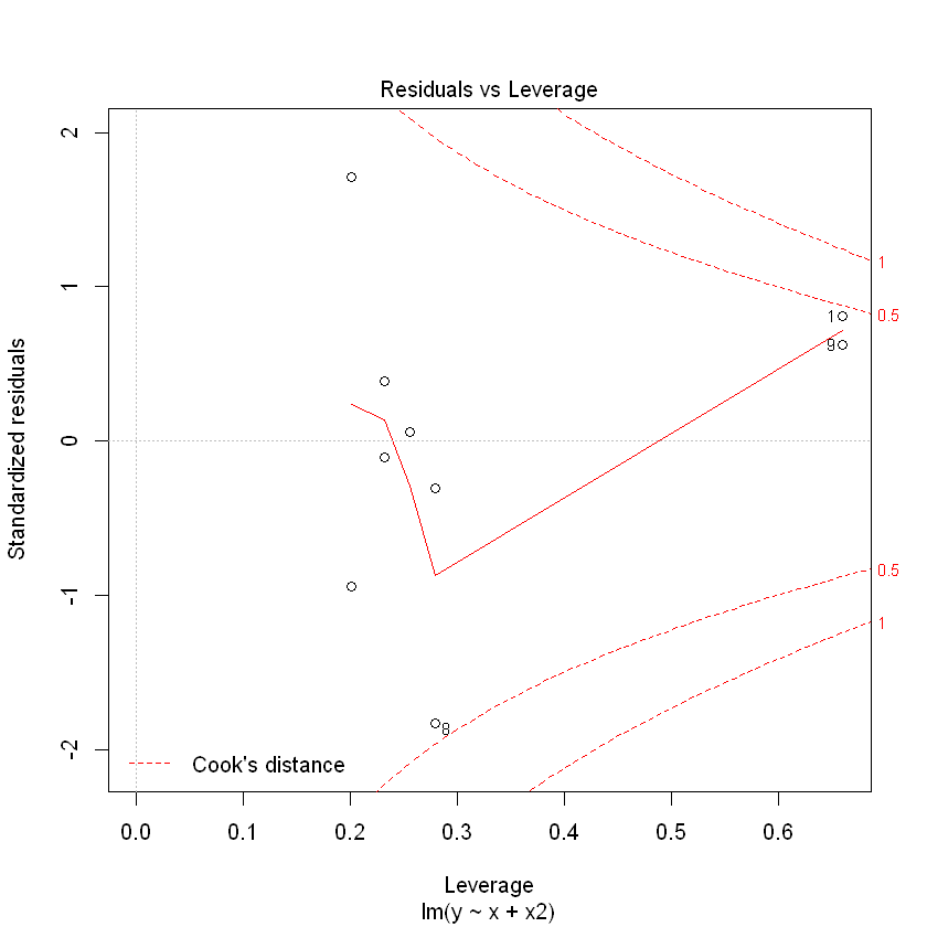
## 2) 제곱항 포함 회귀식 적합
model2 = lm(y~x+x2, df)
summary(model2)
plot(model2)
Call:
lm(formula = y ~ x + x2, data = df)

Residuals:
    Min      1Q  Median      3Q     Max
-0.9606 -0.1606  0.0303  0.2242  0.9455

Coefficients:
            Estimate Std. Error t value Pr(>|t|)
(Intercept)  7.16667    0.78728   9.103 9.87e-05 ***
x           -2.91212    0.36149  -8.056 0.000196 ***
x2           0.45455    0.03526  12.893 1.34e-05 ***
---
Signif. codes:  0 '***' 0.001 '**' 0.01 '*' 0.05 '.' 0.1 ' ' 1

Residual standard error: 0.6187 on 6 degrees of freedom
Multiple R-squared:  0.9898,	Adjusted R-squared:  0.9864
F-statistic: 292.2 on 2 and 6 DF,  p-value: 1.05e-06
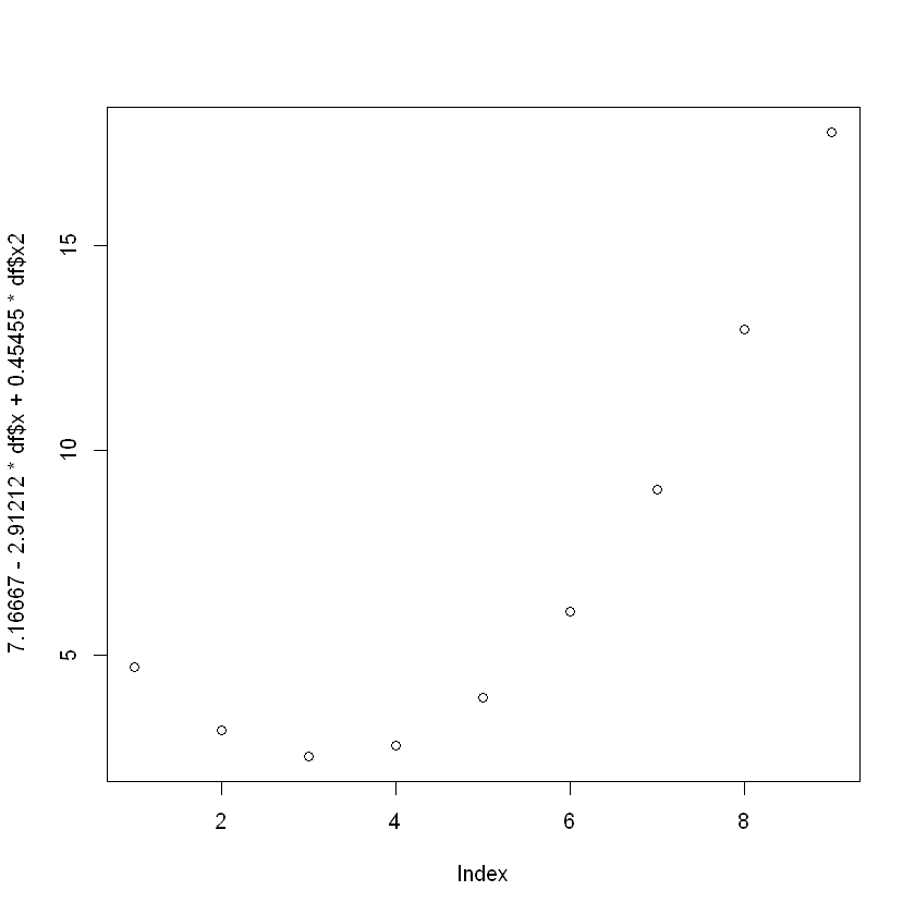
(추정된 회귀식)
y = 7.16667 - 2.91212x + 0.45455x^2
설명력 : 98.98%
(회귀식 잔차도 해석)
model1에 비해 다소 안정된 형태의 잔차를 보임.
plot(7.16667-2.91212*df$x+0.45455*df$x2)
plot(y)
최적회귀방정식의 선택: 설명변수의 선택
(변수선택의 두 가지 원칙)
- y에 영향을 미칠 수 있는 모든 설명변수 x들을 y의 값을 예측하는데 참여시킨다.
- 데이터에 설명변수 x들의 수가 많아지면 관리하는데 많은 노력이 요구되므로,
가능한 범위 내에서 적은 수의 설명변수를 포함시켜야 한다.
- 위 두 가지 원칙은 서로 이율배반적이므로 타협이 이뤄져야 함.
즉, 상황에 적절한 설명변수를 선택해야 함.
1) 모든 가능한 조합의 회귀분석(All possible regression)
AIC(Akaike information criterion)
AIC = 2logL(theta hat) + 2*k
BIC(Bayesian information criterion)
BIC = 2logL(theta hat) + k*log(n)
–> n:자료의 갯수, theta hat:주어진 모형의 모수에 대한 최대가능도 추정량, L(theta hat):가능도함수, k:모형의 모수의 갯수
2) 단계적 변수선택(Stepwise Variable Selection)
- 전진선택법(forward selection)
절편만 있는 상수모형으로부터 시작해 중요하다고 생각되는 설명변수부터 차례로 모형에 추가함.
추가할 수 있는 후보가 되는 설명변수 중 모형에 추가했을 때 가장 제곱합의 기준으로 가장 설명을 잘하는 변수를 고려하여 그 변수가 유의하면 추가하고 그렇지 않은 경우는 추가를 멈춤.
- 후진선택법(backward selection)
독립변수 후보 모두를 포함한 모형에서 출발해 제곱합의 기준으로 가장 적은 영향을 주는 변수부터 하나씩 제거하면서 더 이상 유의하지 않은 변수가 없을 때까지 설명변수들을 제거하고, 이 때의 모형을 선택함.
- 단계별방법(stepwise method)
전진선택법에 의해 변수를 추가하면서 새롭게 추가된 변수에 기인해 기존 변수가 그 중요도가 약화되면 해당변수를 제거하는 등 단계별로 추가 또는 제거되는 변수의 여부를 검토해 더 이상 없을 때 중단함.
(예제) 선형회귀모형 설정 및 후진제거법 통한 변수선택
X1 = c(7,1,11,11,7,11,3,1,2,21,1,11,10)
X2 = c(26,29,56,31,52,55,71,31,54,47,40,66,68)
X3 = c(6,15,8,8,6,9,17,22,18,4,23,9,8)
X4 = c(60,52,20,47,33,22,6,44,22,26,34,12,12)
Y = c(78.5,74.3,104.3,87.6,95.9,109.2,102.7,72.5,93.1,115.9,83.8,113.3,109.4)

df = data.frame(X1,X2,X3,X4,Y)
print(df)
   X1 X2 X3 X4     Y
1   7 26  6 60  78.5
2   1 29 15 52  74.3
3  11 56  8 20 104.3
4  11 31  8 47  87.6
5   7 52  6 33  95.9
6  11 55  9 22 109.2
7   3 71 17  6 102.7
8   1 31 22 44  72.5
9   2 54 18 22  93.1
10 21 47  4 26 115.9
11  1 40 23 34  83.8
12 11 66  9 12 113.3
13 10 68  8 12 109.4
model1 = lm(Y~X1+X2+X3+X4, df)
summary(model1)                      # X3 의 유의확률이 가장 높으므로 제거
Call:
lm(formula = Y ~ X1 + X2 + X3 + X4, data = df)

Residuals:
    Min      1Q  Median      3Q     Max
-3.1750 -1.6709  0.2508  1.3783  3.9254

Coefficients:
            Estimate Std. Error t value Pr(>|t|)
(Intercept)  62.4054    70.0710   0.891   0.3991
X1            1.5511     0.7448   2.083   0.0708 .
X2            0.5102     0.7238   0.705   0.5009
X3            0.1019     0.7547   0.135   0.8959
X4           -0.1441     0.7091  -0.203   0.8441
---
Signif. codes:  0 '***' 0.001 '**' 0.01 '*' 0.05 '.' 0.1 ' ' 1

Residual standard error: 2.446 on 8 degrees of freedom
Multiple R-squared:  0.9824,	Adjusted R-squared:  0.9736
F-statistic: 111.5 on 4 and 8 DF,  p-value: 4.756e-07
model2 = lm(Y~X1+X2+X4, df)
summary(model2)                      # X4 의 유의확률이 가장 높으므로 제거
Call:
lm(formula = Y ~ X1 + X2 + X4, data = df)

Residuals:
    Min      1Q  Median      3Q     Max
-3.0919 -1.8016  0.2562  1.2818  3.8982

Coefficients:
            Estimate Std. Error t value Pr(>|t|)
(Intercept)  71.6483    14.1424   5.066 0.000675 ***
X1            1.4519     0.1170  12.410 5.78e-07 ***
X2            0.4161     0.1856   2.242 0.051687 .
X4           -0.2365     0.1733  -1.365 0.205395
---
Signif. codes:  0 '***' 0.001 '**' 0.01 '*' 0.05 '.' 0.1 ' ' 1

Residual standard error: 2.309 on 9 degrees of freedom
Multiple R-squared:  0.9823,	Adjusted R-squared:  0.9764
F-statistic: 166.8 on 3 and 9 DF,  p-value: 3.323e-08
model3 = lm(Y~X1+X2, df)
summary(model3)
Call:
lm(formula = Y ~ X1 + X2, data = df)

Residuals:
   Min     1Q Median     3Q    Max
-2.893 -1.574 -1.302  1.363  4.048

Coefficients:
            Estimate Std. Error t value Pr(>|t|)
(Intercept) 52.57735    2.28617   23.00 5.46e-10 ***
X1           1.46831    0.12130   12.11 2.69e-07 ***
X2           0.66225    0.04585   14.44 5.03e-08 ***
---
Signif. codes:  0 '***' 0.001 '**' 0.01 '*' 0.05 '.' 0.1 ' ' 1

Residual standard error: 2.406 on 10 degrees of freedom
Multiple R-squared:  0.9787,	Adjusted R-squared:  0.9744
F-statistic: 229.5 on 2 and 10 DF,  p-value: 4.407e-09
위 과정의 후진제거법을 자동으로 실행
step(lm(종속변수~설명변수, 데이터세트), scope=list(lower=~1, upper=~설명변수), direction=”변수선택방법”)
# 후진제거법
step(lm(Y~X1+X2+X3+X4, df), scope=list(lower=~1, upper=~X1+X2+X3+X4), direction = "backward")
Start:  AIC=26.94
Y ~ X1 + X2 + X3 + X4

       Df Sum of Sq    RSS    AIC
- X3    1    0.1091 47.973 24.974
- X4    1    0.2470 48.111 25.011
- X2    1    2.9725 50.836 25.728
<none>              47.864 26.944
- X1    1   25.9509 73.815 30.576

Step:  AIC=24.97
Y ~ X1 + X2 + X4

       Df Sum of Sq    RSS    AIC
<none>               47.97 24.974
- X4    1      9.93  57.90 25.420
- X2    1     26.79  74.76 28.742
- X1    1    820.91 868.88 60.629


Call:
lm(formula = Y ~ X1 + X2 + X4, data = df)

Coefficients:
(Intercept)           X1           X2           X4
    71.6483       1.4519       0.4161      -0.2365
# 전진선택법
step(lm(Y~1, df), scope=list(lower=~1, upper=~X1+X2+X3+X4), direction = "forward")
Start:  AIC=71.44
Y ~ 1

       Df Sum of Sq     RSS    AIC
+ X4    1   1831.90  883.87 58.852
+ X2    1   1809.43  906.34 59.178
+ X1    1   1450.08 1265.69 63.519
+ X3    1    776.36 1939.40 69.067
<none>              2715.76 71.444

Step:  AIC=58.85
Y ~ X4

       Df Sum of Sq    RSS    AIC
+ X1    1    809.10  74.76 28.742
+ X3    1    708.13 175.74 39.853
<none>              883.87 58.852
+ X2    1     14.99 868.88 60.629

Step:  AIC=28.74
Y ~ X4 + X1

       Df Sum of Sq    RSS    AIC
+ X2    1    26.789 47.973 24.974
+ X3    1    23.926 50.836 25.728
<none>              74.762 28.742

Step:  AIC=24.97
Y ~ X4 + X1 + X2

       Df Sum of Sq    RSS    AIC
<none>              47.973 24.974
+ X3    1   0.10909 47.864 26.944


Call:
lm(formula = Y ~ X4 + X1 + X2, data = df)

Coefficients:
(Intercept)           X4           X1           X2
    71.6483      -0.2365       1.4519       0.4161
# 단계선택법
step(lm(Y~1, df), scope=list(lower=~1, upper=~X1+X2+X3+X4), direction = "both")
Start:  AIC=71.44
Y ~ 1

       Df Sum of Sq     RSS    AIC
+ X4    1   1831.90  883.87 58.852
+ X2    1   1809.43  906.34 59.178
+ X1    1   1450.08 1265.69 63.519
+ X3    1    776.36 1939.40 69.067
<none>              2715.76 71.444

Step:  AIC=58.85
Y ~ X4

       Df Sum of Sq     RSS    AIC
+ X1    1    809.10   74.76 28.742
+ X3    1    708.13  175.74 39.853
<none>               883.87 58.852
+ X2    1     14.99  868.88 60.629
- X4    1   1831.90 2715.76 71.444

Step:  AIC=28.74
Y ~ X4 + X1

       Df Sum of Sq     RSS    AIC
+ X2    1     26.79   47.97 24.974
+ X3    1     23.93   50.84 25.728
<none>                74.76 28.742
- X1    1    809.10  883.87 58.852
- X4    1   1190.92 1265.69 63.519

Step:  AIC=24.97
Y ~ X4 + X1 + X2

       Df Sum of Sq    RSS    AIC
<none>               47.97 24.974
- X4    1      9.93  57.90 25.420
+ X3    1      0.11  47.86 26.944
- X2    1     26.79  74.76 28.742
- X1    1    820.91 868.88 60.629


Call:
lm(formula = Y ~ X4 + X1 + X2, data = df)

Coefficients:
(Intercept)           X4           X1           X2
    71.6483      -0.2365       1.4519       0.4161
# 적용

library(MASS)
data(hills)
print(head(hills))
             dist climb   time
Greenmantle   2.5   650 16.083
Carnethy      6.0  2500 48.350
Craig Dunain  6.0   900 33.650
Ben Rha       7.5   800 45.600
Ben Lomond    8.0  3070 62.267
Goatfell      8.0  2866 73.217
model = step(lm(time~1, hills), scope = list(lower=~1, upper=~dist+climb), direction = 'both')
summary(model)
Start:  AIC=274.88
time ~ 1

        Df Sum of Sq   RSS    AIC
+ dist   1     71997 13142 211.49
+ climb  1     55205 29934 240.30
<none>               85138 274.88

Step:  AIC=211.49
time ~ dist

        Df Sum of Sq   RSS    AIC
+ climb  1      6250  6892 190.90
<none>               13142 211.49
- dist   1     71997 85138 274.88

Step:  AIC=190.9
time ~ dist + climb

        Df Sum of Sq     RSS    AIC
<none>                6891.9 190.90
- climb  1    6249.7 13141.6 211.49
- dist   1   23042.0 29933.8 240.30


Call:
lm(formula = time ~ dist + climb, data = hills)

Residuals:
    Min      1Q  Median      3Q     Max
-16.215  -7.129  -1.186   2.371  65.121

Coefficients:
             Estimate Std. Error t value Pr(>|t|)
(Intercept) -8.992039   4.302734  -2.090   0.0447 *
dist         6.217956   0.601148  10.343 9.86e-12 ***
climb        0.011048   0.002051   5.387 6.45e-06 ***
---
Signif. codes:  0 '***' 0.001 '**' 0.01 '*' 0.05 '.' 0.1 ' ' 1

Residual standard error: 14.68 on 32 degrees of freedom
Multiple R-squared:  0.9191,	Adjusted R-squared:  0.914
F-statistic: 181.7 on 2 and 32 DF,  p-value: < 2.2e-16
댓글남기기